Virtual species are often used in ecology to test modelling methods. In my research, I am using virtual species to test species distribution models, but some of the initial work that I am doing involves understanding methods for implementing these simulations. A lot of the work that I do uses Cellular Automata and Individual-Based Models to incorporate processes such as dispersal and population dynamics. However, when developing my own models I quickly found that computational processing time is a big bottleneck.

My development was in Python, which I am use regularly. But I have been putting off for some time the inevitable need dive into lower-level languages such as C and C++ to get the computational performance I needed in my simulations. This avoidance hinged on that fact that I have 3 young kids and doing my PhD, meaning the time needed to learn the intricacies of these languages is non-existent. As an alternative, I decided to give Julia a try and I am really glad that I did. It had a familiar syntax, my code was easily readable and fast! There are still plenty of nuances to the language that I need to brush up on, but as a novice, I can see huge benefits of using Julia.

This post is giving an overview of my “Hellow World” in Julia, where I set out to convert simple cellular automata written in Python. I’ll show how the same model can be implemented in the two different languages and how they both perform in terms of outputs and processing time.

Overview of virtual species

The most common approach to simulating virtual species distributions are:

1. Obtain spatial environmental variables (rasters)

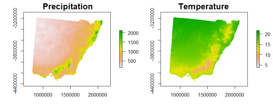
2. Define a habitat suitability function using environmental variables

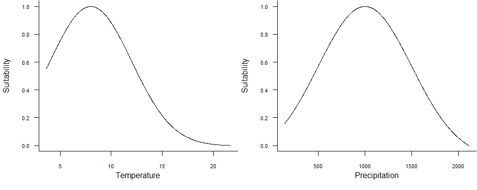
3. Project this function onto 2D space (raster)

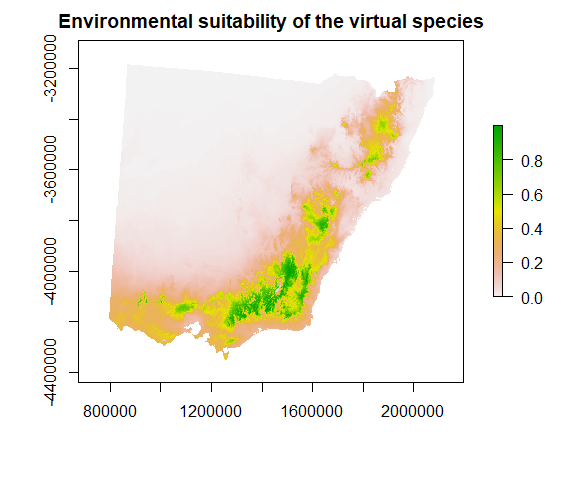
4. Convert habitat suitability into the species response

Typically, the type of response we want to simulate is occurrence (although we could also look to simulate occupancy or abundance). When simulating species occurrence, the suitability function is scaled between zero and one and used to weight Bernoulli trials at each pixel. This produces a stochastic realisation of species occurrence with higher rates of occurrence at cells with high habitat suitability values and low rates where habitat suitability is low.

A more in-depth, practical overview of this process is available here, with the following paper giving valuable perspectives on the topic Meynard, C. N., Leroy, B., & Kaplan, D. M. (2019). Testing methods in species distribution modelling using virtual species: what have we learnt and what are we missing?. Ecography, 42(12), 2021-2036.

The cellular automaton

Many virtual species experiments also try to incorporate endogenous processes (e.g. dispersal) into their simulations. One way to do this is using a cellular automata where each cell the 2D grid takes has a state and the model has a set of rules that determine how these states change over time.

In this model the state a cell can be is either occupied (1) or unoccupied (0). We still use habitat suitability and scale it between zero and one, but it is used as the probability of persistence at each time step. This will be used in the extinction process described later. To incorporate dispersal, occupied cells can produce and propagule and convert a nearby cell to occupied; this is controlled by the colonise process.

To implement this model, I first want to define a constructor to hold the parameters and data required for my cellular automaton.

using Distributions
using DelimitedFiles
using Random
using StatsBase
using Plots

struct OccurenceCellularAutomata
    pa::Array                     # 2D array that can be 0 (un-occupied) or 1 (occupied)
    pa_cart_index::Array          # Index to reference cells in the landscape
    suitability::Array            # 2D array containing scaled suitability values
    dispersalProbability::Float64 # Probability that a cell will disperse at each time step
    meanDispersal::Float64        # Mean dispersal distance
end

Colonisation

During colonisation, a random subset of occupied cells is selected using a binomial distribution to determine how many cells are going to disperse. This controlled by two parameters, first n = the number of occupied cells and p = the dispersal probability.

function selectProportion(pa,caIndex,dispersalProbability)
    nPresences = Int(sum(pa))
    total = Array{CartesianIndex}(undef, nPresences)
    counter = 1
    for idx in caIndex
        if pa[idx] === 1.0
            total[counter] = idx
            counter+=1
        end
    end
    numberDispersing = sample(total,rand(Binomial(nPresences,dispersalProbability)))
end

Each cell that is selected to disperse can then produce one propagule that can colonise a nearby cell using an exponential dispersal kernel. This works by randomly selecting a distance from an exponential distribution and a direction from a uniform distribution between 0 and 360. This is then converted to the nearest integer for both x and y coordinates to give the cell index that is to be colonised. To keep things simple, I don’t check if the cell is already colonised. If a cell is already colonised (i.e.pa[idx] == 1), then it remains that way.

function newPos(meanDistance,cartIdx)
    distance = rand(Exponential(meanDistance),1)
    # + 0.75 ensures dispersal outside of the initial cell
    distance = distance[1] + 0.75
    angle = 360.0*rand()
    # Remember 1 = y, 2 = x
    x = Int(round(cos(deg2rad(angle))*distance,digits=0)) + cartIdx[2]
    y = Int(round(sin(deg2rad(angle))*distance,digits=0)) + cartIdx[1]
    return(y,x)
end
function colonise(ca::OccurenceCellularAutomata)
    shape = size(ca.pa)
    dCells = selectProportion(ca.pa,ca.pa_cart_index,ca.dispersalProbability)
    for i in dCells
        newXY = newPos(ca.meanDispersal,i)
        if newXY[2]>=1 && newXY[2] <= shape[2] && newXY[1] >=1 && newXY[1]<=shape[1]
            ca.pa[newXY[1],newXY[2]] = 1
        end
    end
end

We can run a simple test to make sure the dispersal kernel works as intended with four different mean dispersal distances. This just randomly selects a cell 1,000,000 times and increments the selected cell value each time. We should get a nice circular distribution with high values (yellow) near the centre and low values (blue/purple) towards the outside. I’ll trial four different mean dispersal distances to show how this affects the dispersal patterns.

function test_exponential(dispersal)
    p = zeros(21,21)
    initx = 11
    inity = 11
    for i in 1:1000000
        pos = newPos(dispersal,CartesianIndex(initx,inity))
        if pos[1]>=1 && pos[1]<=21 && pos[2]>=1 && pos[2]<=21
            p[pos[2],pos[1]] +=1
        end
    end
    return(p)
end
test1 = test_exponential(1)
test3 = test_exponential(3)
test6 = test_exponential(6)
test12 = test_exponential(12)
plot(heatmap(test1,c = :viridis),heatmap(test3,c = :viridis),heatmap(test6,c = :viridis),heatmap(test12,c = :viridis))

Extinction

The extinction process iterates over all cells and performs a Bernoulli trial at each occupied cell. This Bernoulli trial is weighted by the probability of persistence in the suitability variable in the OccurenceCellularAutomata object. As a result, occupied cells are more likely to stay occupied into the next timestep in higher suitability cells.

function extinction(ca::OccurenceCellularAutomata)
    for idx in ca.pa_cart_index
        if ca.pa[idx] === 1.0
            survived = rand(Bernoulli(ca.suitability[idx]),1)
            if survived[1] === false
                ca.pa[idx] = 0.0
            end
        end
    end
end

Testing

To run a simulation, I provide a 2D array for habitat suitability which is in ASCII format. This is just a simulated landscape using a spatially autocorrelated Gaussian random field. To initialise the simulation, I set all cells as being occupied and run 200 iterations.

function simulate(ca::OccurenceCellularAutomata,iterations)
    for i in 1:iterations
        colonise(ca)
        extinction(ca)
    end
end
landscape = readdlm("D:/PHDExperimentOutputs/SimLandscapes/suitability/LLM1_suitability.asc",skipstart=6)
ls_dimension = size(landscape)
suit = landscape./100
pa = ones(ls_dimension)
pa_cart_index = CartesianIndices(pa)
dispersalProbability = 0.8
distance = 1.0
simulationModel = OccurenceCellularAutomata(pa,pa_cart_index,suit,dispersalProbability,distance)
n_iterations = 100
@time simulate(simulationModel,n_iterations)
open("D:/test/outJULIA.asc","w") do io
    write(io,"NCOLS 400\nNROWS 400\nXLLCORNER 0\nYLLCORNER 0\nCELLSIZE 100\nNODATA_value -9999\n")
    writedlm(io,simulationModel.pa)
end

  Processing time (Julia): 3.404363s

Comparison to Python

This code was developed by implementing an existing cellular automaton that I had developed in Python. The Python version looks very similar, using a similar number of lines of code but using a class structure.

import numpy as np 
import math,time,array
from numba import jit
from timeit import default_timer as timer

class CA(object):
    def __init__(self,initRaster,suitability,dispersalProbability,meanDist):
        self.suitability = suitability
        self.shape = np.shape(self.suitability)
        self.pa = initRaster
        self.dispersalProbability=dispersalProbability
        self.meanDistance = meanDist
    def newPos(self,x,y):
        distance=np.random.exponential(self.meanDistance,1)
        distance = distance[0] + 0.75
        angle = np.random.uniform(0,360,1)
        newx = int(round(math.cos(math.radians(angle[0])) * distance)) + x
        newy = int(round(math.sin(math.radians(angle[0])) * distance)) + y
        return(newx,newy)
    def selectProportionDispersers(self):
        nPresence = np.sum(self.pa)
        p = np.where(self.pa==1)
        nDispersers = np.random.binomial(nPresence,self.dispersalProbability)
        pID = np.arange(len(p[0]))
        disperserID = np.random.choice(pID,nDispersers,replace=False)
        return([p[0][disperserID],p[1][disperserID]])
    def colonise(self):
        dispersers = self.selectProportionDispersers()
        for i in range(0,len(dispersers[0])):
            pos = self.newPos(dispersers[0][i],dispersers[1][i])
            if pos[0] >= 0 and pos[0] <self.shape[0] and pos[1]>=0 and pos[1]<self.shape[1]:
                self.pa[pos[0],pos[1]] = 1
    def extinction(self):
        p = np.where(self.pa==1)
        for i in range(0,len(p[0])):
            suit = self.suitability[p[0][i]][p[1][i]]
            self.pa[p[0][i]][p[1][i]] = np.random.binomial(1,suit)
    def iterate(self):
        self.colonise()
        self.extinction()

Let’s see how they compare in terms of processing time and whether outputs are comparable or not.

landscape = np.genfromtxt("D:\\PHDExperimentOutputs\\SimLandscapes\\suitability\\LLM1_suitability.asc",delimiter=" ",skip_header=6)/100
header = ''
with open("D:\\PHDExperimentOutputs\\SimLandscapes\\suitability\\LLM1_suitability.asc") as f:
    for i in range(0,6):
        header = header+ f.readline()
height,width = np.shape(landscape) 
initPA = np.ones((height,width))
prob = 0.8
dist = 1
caModel = CA(initPA,landscape,prob,dist)
nIterations = 100
start = timer()
for i in range(0,nIterations):
    caModel.iterate()
end = timer()
print(end-start)
np.savetxt('D:\\test\\outPython.asc',caModel.pa,delimiter=" ",header=header,comments='')

Processing time (Python): 34.30849959999614s

julia_out = readdlm("D:/test/outJULIA.asc",skipstart=6)
python_out = readdlm("D:/test/outPython.asc",skipstart=6)
plot(heatmap(julia_out),heatmap(python_out),size=(1000,400),title=["Julia" "Python"])

While the outputs have differences due to the stochastic nature of the simulations, they both show broadly similar distributional patterns of occurrence. However, if we look at the computational processing time, Julia is hands down the winner at 3.4s compared to 34.3s of Python.

But Python has an ace up its sleeve with Numba, a package that converts Python into optimised machine code to boost performance. It is really simple to use by decorating functions with @jit, although I needed to make a few tweaks to the class structure to make it work.

@jit(nopython=True)
def newPos(meanDistance,x,y):
    distance=np.random.exponential(meanDistance,1)
    distance = distance[0] + 0.75
    angle = np.random.uniform(0,360,1)
    newx = int(round(math.cos(math.radians(angle[0])) * distance)) + x
    newy = int(round(math.sin(math.radians(angle[0])) * distance)) + y
    return(newx,newy)
@jit(nopython=True)
def selectProportionDispersers(pa,dispersalProbability):
    nPresence = np.sum(pa)
    p = np.where(pa==1)
    nDispersers = np.random.binomial(nPresence,dispersalProbability)
    pID = np.arange(len(p[0]))
    disperserID = np.random.choice(pID,nDispersers,replace=False)
    return([p[0][disperserID],p[1][disperserID]])

@jit(nopython=True)
def _colonise(pa,shape,dispersalProbability,distance):
    dispersers = selectProportionDispersers(pa,dispersalProbability)
    for i in range(0,len(dispersers[0])):
        pos = newPos(distance,dispersers[0][i],dispersers[1][i])
        if pos[0] >= 0 and pos[0] <shape[0] and pos[1]>=0 and pos[1]<shape[1]:
            pa[pos[0],pos[1]] = 1

@jit(nopython=True)
def _extinction(suitability,pa):
    p = np.where(pa==1)
    for i in range(0,len(p[0])):
        suit = suitability[p[0][i]][p[1][i]]
        pa[p[0][i]][p[1][i]] = np.random.binomial(1,suit)
    #return(pa)
class CA(object):
    def __init__(self,initRaster,suitability,dispersal_prob,dist):
        self.suitability = suitability
        self.shape = np.shape(self.suitability)
        self.pa = initRaster
        self.dispersal_prob=dispersal_prob
        self.dist = dist
    def colonise(self):
        _colonise(self.pa,self.shape,self.dispersal_prob,self.dist)
    def extinction(self):
        _extinction(self.suitability,self.pa)
    def iterate(self):
        self.colonise()
        self.extinction()

start = timer()
for i in range(0,nIterations):
    caModel.iterate()
end = timer()
print(end-start)
np.savetxt('D:\\test\\outNumba.asc',caModel.pa,delimiter=" ",header=header,comments='')

Processing time (Numba): 2.2075179000094067s

numba_out = readdlm("D:/test/outNumba.asc",skipstart=6)
plot(heatmap(julia_out),size=(430,400),title="Python + Numba")

Turns out Python with Numba is actually faster than Julia, and doesn’t seem to have affected our model, producing a comparable output.

The use of Numba and potentially other tools like PyPY make fast computational processing in Python viable, without the need to switch to Julia. While I will undoubtedly use these tools in future work, using them does raise some issues as they aren’t fully compatible with all Python packages out there. This could lead to issues down the track as I look to share code or possibly develop simulation tools for others to use. Julia on the other hand just works fast straight out the box.

Final thoughts

Julia is a comparatively young language compared to R and Python and the ecosystem of tools is still developing, especially for spatial analysis. This means that it isn’t going to displace these tools for my core work anytime soon. But, as I develop more simulation models such as what I have shown here, I will likely turn to Julia first. The ability to focus on the logic of the model and readability of the code, rather than getting bogged down in the fine details of using lower-level languages is a real advantage. With that said, there are still plenty of concepts in Julia that I still need to get a better grasp of to really get the most of this language.

Julia isn’t going to replace R or Python anytime soon, but looks like a great addition to the toolbox!